Condenser Chemistry Management: From Grab Samples to Predictive Digital Twins

When I walk into the main office of a power plant, it’s always on the main TV screen, along with heat rate, load, and other critical numbers. I’m talking about condenser backpressure. Every power plant manager watches this number (Figure 1), and they should. A PEPSE (Performance Evaluation of Power System Efficiencies) analysis of a 525-MW unit found that each 0.1 inch of mercury absolute (HgA) rise in backpressure raised heat rate by about 0.17%. A 0.3-inch HgA excess in backpressure on a base-loaded unit corresponded to a 2.68-MW power loss and roughly $770,000 in lost revenue. But what information does this single number hold?

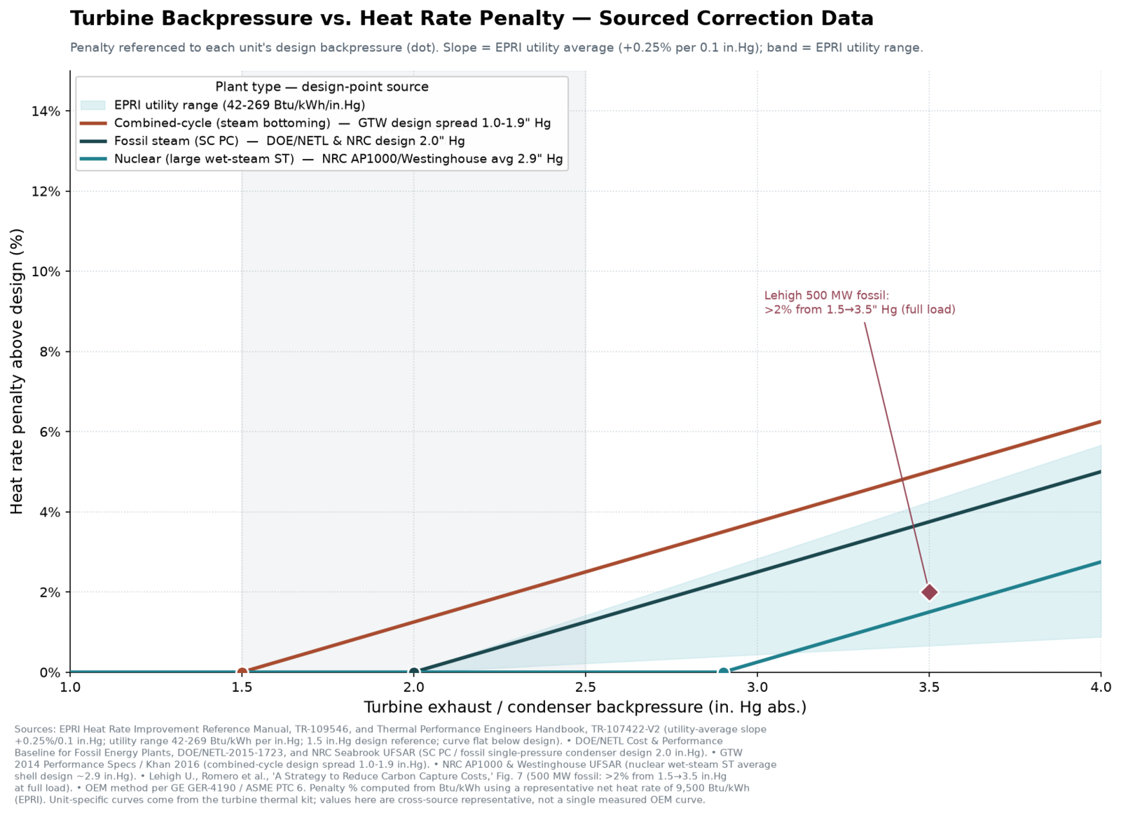
The condenser is where the steam cycle finishes with steam condensed back into water. It’s the largest heat rejection surface in the plant, cooled by water that contains dissolved minerals, suspended solids, organics, and microorganisms; all of which love attaching to a hot tube surface. When that happens, thermodynamics are unforgiving. Waterside deposits raise tube thermal resistance, the condensing temperature climbs, and backpressure rises. This results in the last stages of the turbine burning more fuel per kilowatt-hour to maintain load and the associated rise in heat rate. If it’s severe enough, megawatts drop as the plant can’t maintain production. The Department of Energy estimates that losses are more than $1 billion annually across the U.S. fossil fleet.

Those are big numbers for what amounts to millimeters or less of deposits. The good news is that while thermodynamics haven’t changed, how we precisely see, predict, and control chemistry has seen a dramatic shift in the last 20 years—from grab samples and failure inspections, to traced chemistry and U-coefficient/cleanliness monitoring, and now the implementation of predictive digital twins. We’ll explore the improvements and fidelity associated with the advancements, and what you can implement now to take a step forward in your operation.

The Condenser Is a Chemistry Asset That Bills in Btu/kWh

Heat transfer and resistance live inside the condenser tube where most of the resistance is attributed to water-side factors, which is why the water-side management is so critical. In power plants, heat transfer is typically affected by either scale or microbiological growth. While corrosion can be a factor, the upgraded metallurgies found in most condensers typically negate issues with corrosion. Yes, yellow metals and some stainless still need special care, but let’s focus on scale and microbial growth.

Calcium carbonate, a common deposit in these systems, has a thermal conductivity of 2.26–2.93 watts per meter-kelvin (W/m-K). Biofilm exhibits thermal conductivity of 0.63 W/m-K. Biofilm is roughly 4–5 times more insulating than inorganic salt deposits. A 250-micron layer of biofilm has been reported to cut heat transfer by as much as 50%. 250 microns is the same thickness as three sheets of paper. If you open the condenser, you won’t easily see it, and if you leave it open to dry, you’ll only find non-representative flaky material if you find anything at all.

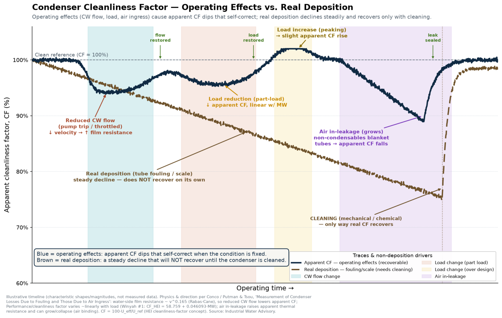
Cleanliness factor—the ratio of the actual overall heat transfer coefficient to the clean design coefficient, calculated by the Heat Exchange Institute method—is currently the benchmark standard in understanding cleanliness while online (Figure 2). A clean condenser put into service typically achieves a cleanliness factor of 85% or higher. This becomes the baseline for “clean.” Cleanliness factor can be a primary gauge for how well your water treatment is performing. Trending cleanliness factor over time allows you to have a surrogate for how close to clean you are maintaining the condenser. But a few things to consider: cleanliness factor will shift with changing load, air ingress and blanketing, and cooling water velocity. This means complex normalization and refactoring are typically required to maintain an understanding. It’s not a straightforward measurement like backpressure.

So, what about monitoring, control, predictivity, and chemistry impacts? And how does that tie to backpressure or cleanliness factor? We still use chemicals, we still use pumps, we still take grab samples. What’s changed, and what’s new? Over 25 years, I’ve seen power plants that still operate on 40-plus-year-old methods, and those that have adopted the latest capabilities. Let’s get grounded in the improvements in condenser cleanliness management.

Stage 1: Legacy Indices and Grab Samples

Since its invention in 1936, industry has found any number of ways to use Langelier Saturation Index (LSI), or a modern interpretation, Ryznar Stability Index (RSI). Operators already run calcium, alkalinity, pH, conductivity, and other analyses on the water, so calculating LSI was an easy early measure of potential scaling that didn’t require computing power. Couple that approach with corrosion coupons measured at 30, 60, or 90 days, and you had the basis of a water treatment management program.

That approach was rational for the instrumentation available, and it prevented a lot of damage. In fact, most chemical dosage guidance for power applications was based on LSI even into the 2010s. Unfortunately, this approach also carried four structural limitations worth highlighting as we still see problems every day in operating plants.

• LSI Describes Saturation of One Salt, Calcium Carbonate (CaCO₃), in Bulk Water at Bulk Temperature. It was designed for municipal drinking water systems and never intended for industrial systems. Other common salts like calcium phosphate, calcium sulfate, silica, magnesium silicate, or the iron and aluminum interactions that consume water treatment chemicals remain unseen risks.
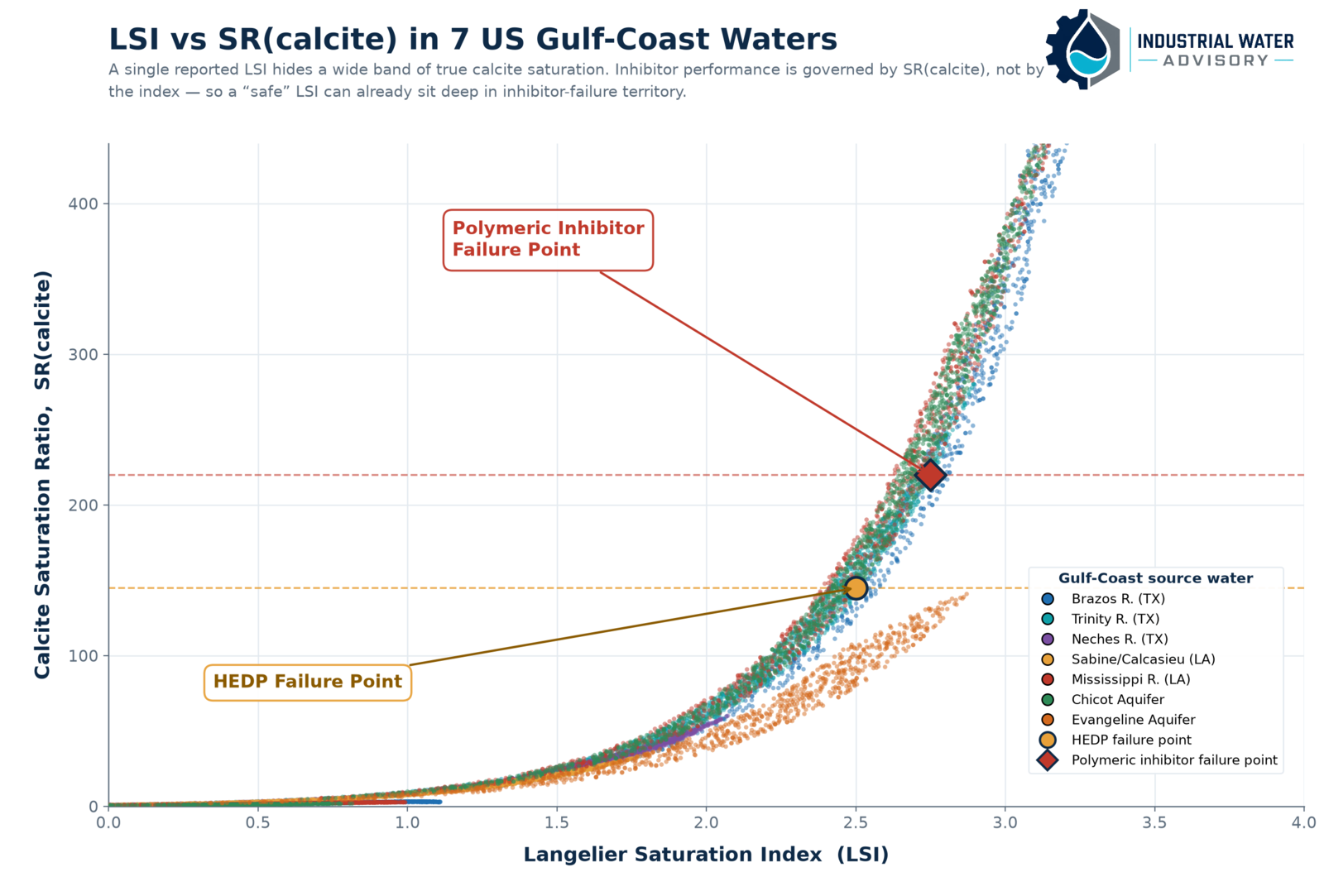
• LSI Was Never a Corrosion Predictor. This is misquoted so much that even Google’s Gemini serves you the wrong answer. It is a common misconception. It is only a measure of the propensity of CaCO₃ to precipitate (positive LSI) or dissolve (negative LSI). It is useful up to approximately +1.3–1.5 LSI. Above this level its correlation with the true calcite (CaCO₃) saturation degrades, which leads to situations where LSI looks controllable with chemistry, but the actual calcite saturation is much higher, leading to deposition and failure conditions (Figure 3).

• LSI Should Never Be Calculated Based on a Grab Sample of Cycled Water Chemistry. If you are actively losing calcium and alkalinity to deposition, calculating LSI on the recirculating water will reflect this lower calcium and alkalinity value, giving you a lower LSI and falsely indicating a better condition than is actually occurring. Always calculate LSI based on a theoretical cycled up value of the makeup water and compare that to the circulating water. This gives you the picture of where the water should be if all constituents are in control and allows you to make better decisions.
• Monthly Sampling Aliases Everything That Moves. Cooling systems are driven by load, wet-bulb, makeup quality, process leaks, cycles excursions, acid excursions, etc.—all of which vary by hours. A grab sample is one point on a curve you cannot see. A plant can operate for two weeks out of spec, depositing in the condenser, and return to target before the next test, falsely indicating that the system was fully in control.

Stage 2: Tagged Chemistry and Online Analyzers

The next advance solved a problem that long plagued the industry. Despite all the wet testing and draw-down column measurements conducted in the field, nobody actually knew how much active chemistry was in the system—or whether the right amount was being applied. Inert fluorescent tracers like PTSA (pyrenetetrasulfonic acid) included in product formulations allow a fluorometer to determine the product concentration in the system in real time, verifying the chemical feed rate.

Tagged polymers then emerged that extended the idea to understanding just how much of a particular active molecule was in the system. These technologies were complemented by online conductivity, ORP (oxidation-reduction potential), pH, corrosion rate, and water meters that helped fill in the gaps. But the real first step toward predictivity was the implementation of side-stream deposit/fouling monitors. Using setpoints the same as or slightly worse than actual operating conditions, these units attempted to predict deposition through real heat transfer on a surface, allowing operators to adjust chemistry before the same conditions occur in the system.

This was a genuine step change, and it delivered three things:

• Feed Accuracy Became Measurable. Pump drift, pluggage, dilution errors, and mis-set stroke lengths were immediately visible. Alarms could be set based on feed accuracy, ensuring feed control was constantly watched and not just reviewed at the next quarterly meeting.
• Precision Economics Can Be Tracked. Take your blowdown rate in gallons per minute (gpm) and multiply by 4.4: that is the pounds of active chemical per year leaving the system for every 1 part per million (ppm) you hold in the circulating water. The arithmetic is just unit conversion—1 gpm is 525,600 gallons per year, about 4.38 million pounds of water, and 1 ppm of that is 4.38 pounds. On a 100,000-gpm circulating system with a 20F range running four cycles of concentration, blowdown is roughly 667 gpm, so every 1 ppm of product feedrate costs about 2,900 pounds of active per year. Carry 4 ppm more than the program requires and you have quietly added five figures of annual spend that no one approved. Run 2 ppm short at the wrong time and you pay for it in cleanliness factor instead. Both errors are calculable, and neither is visible in an index.
• Fouling Stopped Being a Mystery Until the Outage. A cleanliness factor trend paired with a fouling monitor and a chemistry record made it possible to attribute a performance loss to waterside deposit rather than air in-leakage, and to distinguish microfouling from tubesheet macrofouling. It removes much of the complex normalization and refactoring.

But this stage was also the start of a failure mode I see all the time, and initiated a decline in core water treatment knowledge in the industry.

A Tracer Confirms Presence, Not Performance. And a Molecular Tag Confirms the Molecule Was There, but Not Its Current State. I see more and more people being comfortable just checking the tracer and tag, and walking away believing the system is in control. While these are great tools to help you know how much of a product has been fed to a system, you might be walking away from the system with more risk than you realize (Figure 4). Phosphonates are consumed, polymers shear and lose dispersancy, azoles get complexed, and oxidants affect the core chemistry. None of which may affect your tracer/tag level. An on-target tracer with a degrading cleanliness factor is one of the most common challenges I see in condensers today. And the longer these are in practice, the more we see teams trust the tag and question the thermal data, instead of the other way around. These are helpful tools, but not replacements for good engineering and chemical practices.

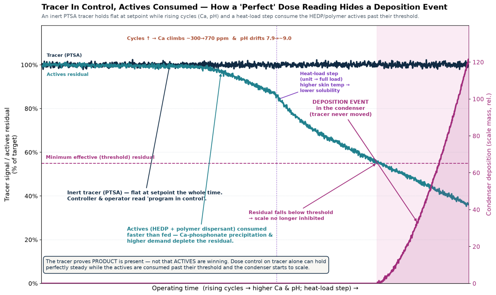
Measurement Is Not Prediction. And let’s remember that we’re still looking at current or historical state here. It tells you something has already changed. You’re chasing the source and trying to play catchup. It doesn’t tell you what’s coming that you should be prepared for.

Stage 3: Progressive Fidelity Digital Twins

The term digital twin has been applied loosely enough that it deserves a working definition for this context. A useful cooling-water twin has three parts:

• A first-principles chemistry model that performs full ion speciation and calculates saturation ratios for all relevant solid phases, along with kinetic rates—carbonate, phosphate, sulfate, silicate, and the iron and aluminum species—accounting for competing ions and ionic strength rather than one index for one salt.
• A thermal-hydraulic model of the heat transfer surface that computes local wall and skin temperature, velocity, and film conditions from live operating data, so the chemistry is evaluated where deposition actually occurs.
• Continuous calibration against measured plant data—cleanliness factor, terminal temperature difference, backpressure, cooling water inlet and outlet temperatures, flow, and the chemistry instrumentation from the previous era—with explicit validation against known outcomes.

Coupling those three is the meaningful step. It moves the saturation calculation from the tower basin to the tube wall, which is the difference between a compliance number and an engineering answer. A twin that reports the calcite and phosphate saturation ratio in the boundary layer of the hottest tube in the bundle at current load is answering the question the plant actually has: is this water depositing right now, on this surface, at these conditions.

Newer models also allow progressive fidelity: you can start with the data that you have and they will show you the accuracy improvement of moving to more sensors or more data. So, you can choose the level you need for your plan decision-making process (Figure 5), without going to a full-blown, multi-hundred-thousand-dollar implementation and massive project right away.

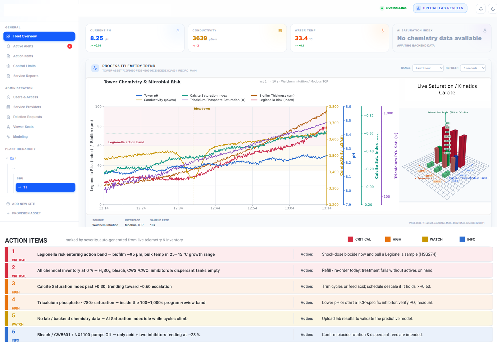
A few important things to note about the current state of digital twins:

• Prediction Is Not Trending. Most of what is marketed today is a historical look at data that then tries to interpret a previously known deviation from that historical pattern. A first-principles twin can simulate a condition the plant has never run: a new makeup blend, six cycles instead of four, five-degree hotter cooling water, or a reduction in chemical inhibitor. Historical data is a calibration point, not something to extrapolate from.
• Data Quality. Engineers have never been short on models. We can develop models for just about anything. Where we fall short is the quality and consistency of data the model receives. The same is true for digital twins. Estimates can be found in error bands. A high-quality model built on estimates or poor data will confidently produce precise, wrong answers, and its precision will make it harder for people to challenge. The quality of the data and data sources are critical.
• It Has to Change a Decision. Twins can deliver beautiful dashboards, but the real measure of value is: does that twin help you to make or change a decision based on its output. Did you change a cleaning cycle? Chemistry setpoint? Cycles Target? Etc.

Making Chemistry a Performance Lever

Put the three stages together and the practical payoff is that chemistry becomes an optimization variable in the same economic frame as fuel and cleaning, rather than a fixed cost defended by a compliance envelope.

Consider the cycles of concentration decision, which nearly every plant treats as settled. Raising cycles cuts makeup and blowdown, saves water, and reduces chemical mass leaving the system—about 4.4 pounds of active per year per gpm of blowdown per ppm, so the savings are directly calculable. It also raises every saturation ratio at the tube wall, shortens the margin before deposition, lengthens holding time, and puts more of the burden on inhibitor performance. Run that trade in an index and you get a yes-or-no answer against a table. Run it in a twin at skin conditions and you get the actual deposition envelope, the inhibitor dosage required to hold it, the chemistry cost of that dosage, and the expected cleanliness factor consequence if you are wrong. One is a rule. The other is an engineering decision with the cost of each branch attached.

The same framing applies to cleaning intervals. Condenser cleaning economics are well understood—the optimization is a balance between cleaning cost and the fuel cost of degraded performance, and EPRI-era work rather than the calendar. What a chemistry-aware twin adds is the ability to forecast the fouling rate as a function of the chemistry you intend to run, rather than measuring it after the fact. That turns an interval into a lever.

And it applies to the argument every plant eventually has with its treatment supplier about whether the program is performing. A cleanliness factor trend, a validated saturation picture at skin conditions, a verified feed record, and a documented blowdown rate turn that conversation from competing opinions into a shared data set. In my experience that shift—from opinion to instrumented, thermodynamically defensible evidence—resolves more disputes than any change in chemistry ever does.

What Good Looks Like

If a plant wants to move up this curve without buying its way into a dashboard it will not use, the sequence that works is unglamorous:

• Measure What the Model Will Depend On. Verified circulating water flow, not a nameplate. Whole-loop volume from drawings and equipment holdup, not basin geometry. Calibrated pH and conductivity, checked against grab samples on a schedule with the results recorded.
• Cross-Check Your Cycles. Compare conductivity-based cycles against a conservative species such as chloride or silica. When they disagree by more than 10% to 15%, stop and find out why. That gap is usually a contaminant ingress or an unmetered loss, and both matter more than the chemistry adjustment you were about to make.
• Put Cleanliness Factor and Chemistry on the Same Page. One trend chart, same time axis, per the American Society of Mechanical Engineers Performance Test Code (ASME PTC) 12.2 methodology for the thermal side. Review both together, monthly, with the treatment provider in the room.
• Separate Feed Assurance from Performance Assurance. Use tags and tracers for what they are good at—confirming feed. Use thermal performance, deposit analysis, and corrosion data to judge whether the chemistry is working. Never let the first substitute for the second.
• Evaluate Saturation and Kinetics Where Deposition Occurs. Move from bulk-water indices to full speciation at tube-skin conditions for the salts your water can actually precipitate. This is the single largest technical upgrade available in cooling water control, and it does not require new chemistry—only a better calculation of the water you already have.
• Validate Before You Trust. Ask any model to reproduce a known past event at your plant—a fouling episode, a cleaning recovery, a cycles excursion—before you let it set a target.

The Direction of Travel

The trajectory here is consistent, and it is not really about software. Cooling water control has moved from describing bulk water occasionally, to measuring feed and residuals continuously, to modeling the chemistry at the surface where it does its damage. Each step narrowed the gap between what we controlled and what actually determined condenser performance.

What has not changed is the burden of proof. A condenser is an instrumented thermodynamic experiment running continuously, and it will tell you whether your chemistry is right if you are willing to read cleanliness factor, terminal temperature difference, and backpressure as chemistry data. The plants that get the most out of this are not the ones with the most sophisticated model. They are the ones that measured their fundamentals honestly, connected chemistry decisions to thermal outcomes, and stopped accepting an in-range index as evidence that the condenser was clean.

Treat the water chemistry as a performance lever and the condenser will pay you in heat rate and megawatts. Treat it as a compliance exercise and it will bill you in the same currency.

—Jim Green is an independent industrial water consultant with 25 years in industrial water treatment, cooling water program design, deposition and corrosion control, and failure analysis for refining, petrochemical, power generation, district cooling, and data center facilities. He can be reached at .